Heart Failure Prediction by Analysing Clinical Records

This project aims to analyze the factors involved in heart failure in patients and develop a model that can predict whether a patient will survive or not.

Dataset

This dataset contains the medical records of 5000 patients who had heart failure, collected during their follow-up period, where each patient profile has 13 clinical features.

Attribute Information:

age: Age of the patient (years)
anaemia: Lack of red blood cells or hemoglobin (boolean)
creatinine_phosphokinase: Level of the CPK enzyme in the blood (mcg/L)
diabetes: Whether the patient has diabetes (boolean)
ejection_fraction: Percentage of blood leaving the heart at each contraction (percentage)
high_blood_pressure: Whether the patient has hypertension (boolean)
platelets: Count of platelets in the blood (kiloplatelets/mL)
sex: Woman or man (binary)
serum_creatinine: Level of serum creatinine in the blood (mg/dL)
serum_sodium: Level of serum sodium in the blood (mEq/L)
smoking: Whether the patient smokes or not (boolean)
time: Follow-up period (days)
DEATH_EVENT: Whether the patient died during the follow-up period (boolean)

Code

### Preparing the data

													#import necessary packages
from imblearn.over_sampling import SMOTE
from scipy.stats import gaussian_kde
from sklearn.cluster import KMeans
from sklearn.decomposition import PCA
from sklearn.ensemble import RandomForestClassifier
from sklearn.linear_model import LogisticRegression
from sklearn.metrics import classification_report,confusion_matrix,accuracy_score
from sklearn.model_selection import GridSearchCV,train_test_split
from sklearn.naive_bayes import GaussianNB
from sklearn.neighbors import KNeighborsClassifier
from sklearn.preprocessing import LabelEncoder
from sklearn.preprocessing import StandardScaler
from sklearn.svm import SVC
from sklearn.tree import DecisionTreeClassifier
import matplotlib.pyplot as plt
import numpy as np
import pandas as pd
import seaborn as sns
import xgboost as xgb

%matplotlib inline
🗸 9.6s
#import data into dataframe
heart_failure_df=pd.read_csv('../data/Heart Failure Prediction - Clinical Records/heart_failure_clinical_records.csv')
heart_failure_df.head()
🗸 0.0s

	age	anaemia	creatinine_phosphokinase	diabetes	ejection_fraction	high_blood_pressure	platelets	serum_creatinine	serum_sodium	sex	smoking	time	DEATH_EVENT
0	55.0	0	748	0	45	0	263358.03	1.3	137	1	1	88	0
1	65.0	0	56	0	25	0	305000.00	5.0	130	1	0	207	0
2	45.0	0	582	1	38	0	319000.00	0.9	140	0	0	244	0
3	60.0	1	754	1	40	1	328000.00	1.2	126	1	0	90	0
4	95.0	1	582	0	30	0	461000.00	2.0	132	1	0	50	1

	heart_failure_df.duplicated(keep=False)
🗸 0.0s 0        True
 1        True
 2        True
 3       False
 4       False
         ...  
 4995     True
 4996     True
 4997     True
 4998     True
 4999     True
 Length: 5000, dtype: bool
    heart_failure_df=heart_failure_df.drop_duplicates()
heart_failure_df.info()
🗸 0.0s <class 'pandas.core.frame.DataFrame'>
 Index: 1320 entries, 0 to 4972
 Data columns (total 13 columns):
  #   Column                    Non-Null Count  Dtype  
 ---  ------                    --------------  -----  
  0   age                       1320 non-null   float64
  1   anaemia                   1320 non-null   int64  
  2   creatinine_phosphokinase  1320 non-null   int64  
  3   diabetes                  1320 non-null   int64  
  4   ejection_fraction         1320 non-null   int64  
  5   high_blood_pressure       1320 non-null   int64  
  6   platelets                 1320 non-null   float64
  7   serum_creatinine          1320 non-null   float64
  8   serum_sodium              1320 non-null   int64  
  9   sex                       1320 non-null   int64  
  10  smoking                   1320 non-null   int64  
  11  time                      1320 non-null   int64  
  12  DEATH_EVENT               1320 non-null   int64  
 dtypes: float64(3), int64(10)
 memory usage: 144.4 KB
 heart_failure_df.describe()
🗸 0.0s

	age	anaemia	creatinine_phosphokinase	diabetes	ejection_fraction	high_blood_pressure	platelets	serum_creatinine	serum_sodium	sex	smoking	time	DEATH_EVENT
count	1320.000000	1320.000000	1320.000000	1320.000000	1320.000000	1320.000000	1320.000000	1320.000000	1320.000000	1320.000000	1320.000000	1320.000000	1320.000000
mean	60.587377	0.485606	576.135606	0.446970	37.881818	0.369697	263751.982189	1.356447	136.665909	0.645455	0.307576	132.678788	0.300758
std	11.913538	0.499982	970.630878	0.497368	11.572547	0.482906	106345.010143	0.998924	4.380990	0.478557	0.461665	77.779493	0.458761
min	40.000000	0.000000	23.000000	0.000000	14.000000	0.000000	25100.000000	0.500000	113.000000	0.000000	0.000000	4.000000	0.000000
25%	50.000000	0.000000	115.000000	0.000000	30.000000	0.000000	208000.000000	0.900000	134.000000	0.000000	0.000000	74.000000	0.000000
50%	60.000000	0.000000	249.000000	0.000000	38.000000	0.000000	263358.030000	1.100000	137.000000	1.000000	0.000000	119.500000	0.000000
75%	69.000000	1.000000	582.000000	1.000000	45.000000	1.000000	310000.000000	1.300000	140.000000	1.000000	1.000000	206.000000	1.000000
max	95.000000	1.000000	7861.000000	1.000000	80.000000	1.000000	850000.000000	9.400000	148.000000	1.000000	1.000000	285.000000	1.000000

 heart_failure_df.mode()
🗸 0.0s

	age	anaemia	creatinine_phosphokinase	diabetes	ejection_fraction	high_blood_pressure	platelets	serum_creatinine	serum_sodium	sex	smoking	time	DEATH_EVENT
0	60.0	0	582	0	35	0	263358.03	1.0	134	1	0	74	0

	heart_failure_df.median()
🗸 0.0s age                             60.00
 anaemia                          0.00
 creatinine_phosphokinase       249.00
 diabetes                         0.00
 ejection_fraction               38.00
 high_blood_pressure              0.00
 platelets                   263358.03
 serum_creatinine                 1.10
 serum_sodium                   137.00
 sex                              1.00
 smoking                          0.00
 time                           119.50
 DEATH_EVENT                      0.00
 dtype: float64
    heart_failure_df=heart_failure_df.astype(
    {
        'age': 'uint8',
        'anaemia': 'bool',
        'creatinine_phosphokinase': 'int16',
        'diabetes': 'bool',
        'ejection_fraction': 'uint8',
        'high_blood_pressure': 'bool',
        'platelets': 'int32',
        'serum_creatinine': 'float32',
        'serum_sodium': 'uint8',
        'sex': 'bool',
        'smoking': 'bool',
        'time': 'uint16',
        'DEATH_EVENT': 'bool'
    }
)
heart_failure_df.info()
🗸 0.0s <class 'pandas.core.frame.DataFrame'>
 Index: 1320 entries, 0 to 4972
 Data columns (total 13 columns):
  #   Column                    Non-Null Count  Dtype  
 ---  ------                    --------------  -----  
  0   age                       1320 non-null   uint8  
  1   anaemia                   1320 non-null   bool   
  2   creatinine_phosphokinase  1320 non-null   int16  
  3   diabetes                  1320 non-null   bool   
  4   ejection_fraction         1320 non-null   uint8  
  5   high_blood_pressure       1320 non-null   bool   
  6   platelets                 1320 non-null   int32  
  7   serum_creatinine          1320 non-null   float32
  8   serum_sodium              1320 non-null   uint8  
  9   sex                       1320 non-null   bool   
  10  smoking                   1320 non-null   bool   
  11  time                      1320 non-null   uint16 
  12  DEATH_EVENT               1320 non-null   bool   
 dtypes: bool(6), float32(1), int16(1), int32(1), uint16(1), uint8(3)
 memory usage: 37.4 KB
 heart_failure_df.memory_usage(deep=True)
🗸 0.0s Index                       10560
 age                          1320
 anaemia                      1320
 creatinine_phosphokinase     2640
 diabetes                     1320
 ejection_fraction            1320
 high_blood_pressure          1320
 platelets                    5280
 serum_creatinine             5280
 serum_sodium                 1320
 sex                          1320
 smoking                      1320
 time                         2640
 DEATH_EVENT                  1320
 dtype: int64

## Exploratory Data Analysis

sns.set_theme(style="darkgrid", palette="pastel")
🗸 0.0s
heart_failure_df.groupby(['DEATH_EVENT']).describe()['age'].transpose()
🗸 0.0s

DEATH_EVENT	False	True
count	923.000000	397.000000
mean	58.824485	64.662469
std	10.723075	13.459326
min	40.000000	40.000000
25%	50.000000	53.000000
50%	60.000000	65.000000
75%	65.000000	72.000000
max	90.000000	95.000000

	#KDE Intersection
def find_kde_intersections(df, feature, death_event_col='DEATH_EVENT',feature_kde_scale=1):
    feature_death_event_0 = df[df[death_event_col] == 0][feature]
    feature_death_event_1 = df[df[death_event_col] == 1][feature]

    kde_death_event_0 = gaussian_kde(feature_death_event_0)
    kde_death_event_1 = gaussian_kde(feature_death_event_1)

    x_values = np.linspace(min(df[feature]), max(df[feature]), 1000)
    y_death_event_0 = kde_death_event_0.evaluate(x_values)
    y_death_event_1 = kde_death_event_1.evaluate(x_values)

    x_intersection_points = []
    y_intersection_points = []

    for i in range(len(x_values) - 1):
        if np.sign(y_death_event_0[i] - y_death_event_1[i]) != np.sign(y_death_event_0[i + 1] - y_death_event_1[i + 1]):
            x_intersect = (x_values[i] + x_values[i + 1]) / 2
            y_intersect = (y_death_event_1[i] + y_death_event_1[i + 1]) / 2
            x_intersection_points.append(x_intersect)
            y_intersection_points.append(y_intersect * feature_kde_scale)

    return x_intersection_points, y_intersection_points, kde_death_event_0, kde_death_event_1
🗸 0.0s
#age distribution
age_kde_scale = (heart_failure_df['age'].mean()*heart_failure_df['age'].std())/2
x_age_intersection_points, y_age_intersection_points, age_kde_death_event_0, age_kde_death_event_1 = find_kde_intersections(heart_failure_df, 'age', feature_kde_scale=age_kde_scale)

plt.figure(figsize=(15,8))
plt.title('Patients older than 69.9 are less likely to survive')

sns.histplot(heart_failure_df,x='age',stat='percent',hue='DEATH_EVENT',kde=True,palette='Set2',multiple='dodge',fill=True, common_norm=False)

plt.legend(['Did not Survive','Survived'])

plt.xlabel('Age')
plt.xticks(range(40,100,5))
plt.xlim(40,95)

plt.ylabel('Survivability %')
plt.yticks(range(0,21))
plt.ylim(0,20)

for i,x_age_point in enumerate(x_age_intersection_points):
    plt.axvline(x_age_point, color='gray', linestyle='--', linewidth=0.75)
    y_age_point = y_age_intersection_points[i]
    plt.text(x_age_point, y_age_point+0.5, f'{x_age_point:.1f}', color='black', rotation=0,va='top', ha='center')
  
plt.show()
🗸 0.0s

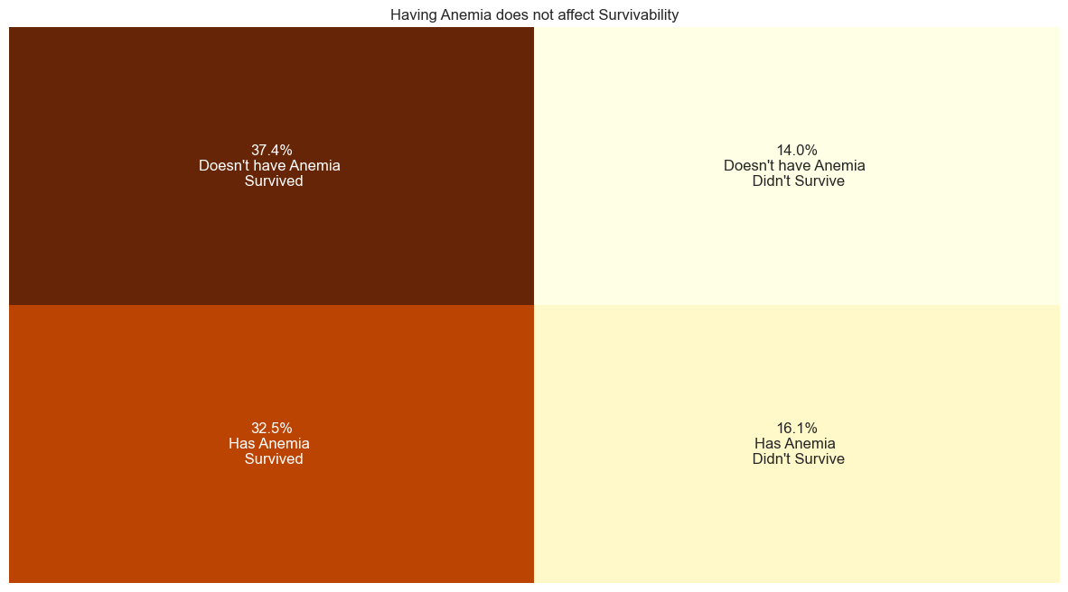
### What is Anemia? Anemia is when you have low levels of healthy red blood cells to carry oxygen throughout your body. ### How much of our patients are Anemic?

#Categorization
def categorize_values(a, b,c):
    if a == 0 and b == 0:
        return f"Doesn't have {c} \n Survived"
    elif a == 0 and b == 1:
        return f"Doesn't have {c} \n Didn't Survive"
    elif a == 1 and b == 0:
        return f"Has {c} \n Survived"
    elif a == 1 and b == 1:
        return f"Has {c} \n Didn't Survive"
    else:
        return 'Undefined'
🗸 0.0s
#anemic distribution
anemic_contingency_table=pd.crosstab(heart_failure_df['anaemia'],heart_failure_df['DEATH_EVENT']).copy()

annotations = [
    [
        '{:.1f}%\n{}'.format(anemic_contingency_table.iloc[i, j] / anemic_contingency_table.sum().sum() * 100, 
                               categorize_values(anemic_contingency_table.index[i], anemic_contingency_table.columns[j], 'Anemia'))
        for j in range(len(anemic_contingency_table.columns))
    ]
    for i in range(len(anemic_contingency_table.index))
]

plt.figure(figsize=(15,8))
plt.title('Having Anemia does not affect Survivability')

sns.heatmap(anemic_contingency_table, annot=annotations, fmt='', cmap='YlOrBr', cbar=False)

plt.xlabel('')
plt.xticks([])

plt.ylabel('')
plt.yticks([])

plt.show()
🗸 0.1s

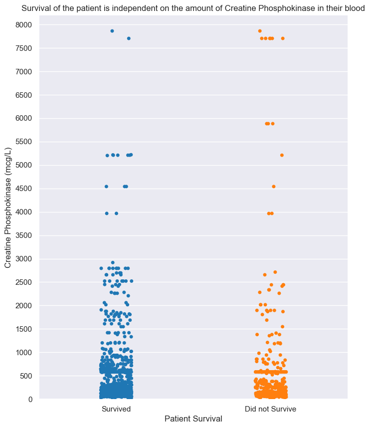
### What is Creatine Phosphokinase (CPK)? Creatine Phosphokinase (CPK) is an enzyme that mainly exists in your heart and skeletal muscle, with small amounts in your brain. ### What Is the Normal Range of CPK Levels? Usually, the normal range of CPK levels falls anywhere between 10 to 120 micrograms per liter (mcg/L). ### How much in our patient?

#cpk distribution
plt.figure(figsize=(8,10))
plt.title('Survival of the patient is independent on the amount of Creatine Phosphokinase in their blood')

sns.stripplot(heart_failure_df,y='creatinine_phosphokinase',x='DEATH_EVENT',hue='DEATH_EVENT',jitter=True,palette='tab10',legend=False)

plt.xlabel('Patient Survival')
plt.xticks([0,1],['Survived','Did not Survive'])

plt.ylabel('Creatine Phosphokinase (mcg/L)')
plt.yticks(range(0,8250,500))
plt.ylim(0,8200)

plt.show()        
🗸 0.2s

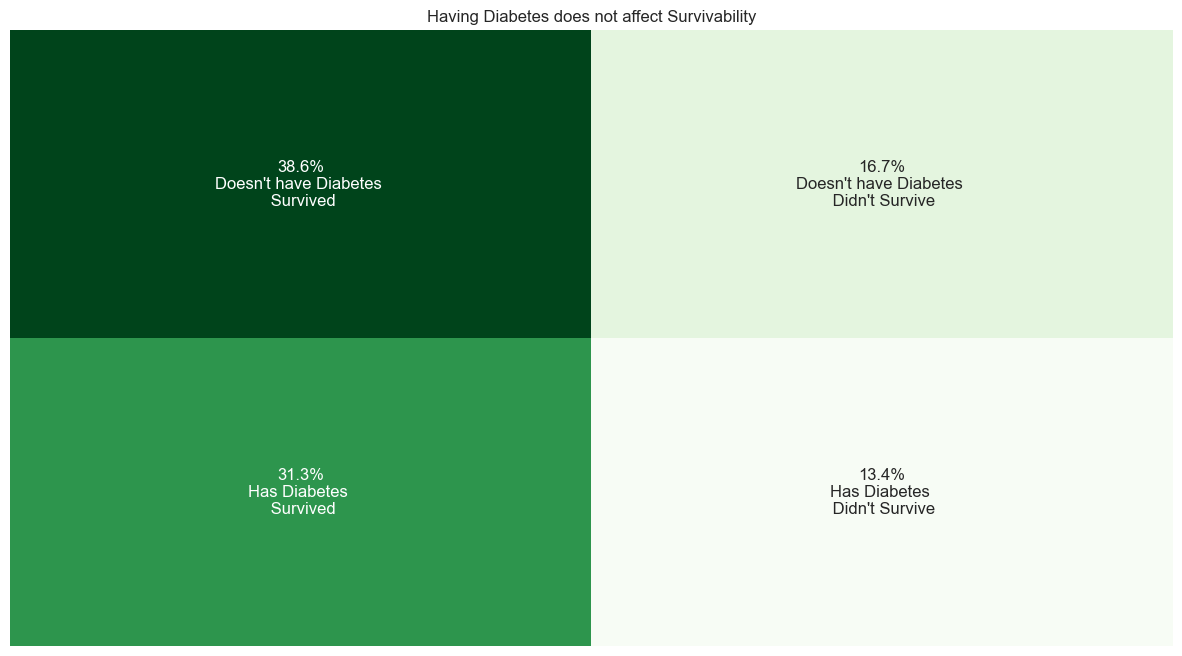
### What is Diabetes? Diabetes is a condition that happens when your blood sugar (glucose) is too high. It develops when your pancreas doesn’t make enough insulin or any at all, or when your body isn’t responding to the effects of insulin properly. ### How much of our patients are Diabetic?

#diabetes distribution
diabetic_contingency_table=pd.crosstab(heart_failure_df['diabetes'],heart_failure_df['DEATH_EVENT']).copy()

annotations = [
    [
        '{:.1f}%\n{}'.format(diabetic_contingency_table.iloc[i, j] / diabetic_contingency_table.sum().sum() * 100,
                             categorize_values(diabetic_contingency_table.index[i], diabetic_contingency_table.columns[j],'Diabetes'))
        for j in range(len(diabetic_contingency_table.columns))
    ]
    for i in range(len(diabetic_contingency_table.index))
]

plt.figure(figsize=(15,8))
plt.title('Having Diabetes does not affect Survivability')

sns.heatmap(diabetic_contingency_table, annot=annotations, fmt='', cmap='Greens', cbar=False)

plt.xlabel('')
plt.xticks([])

plt.ylabel('')
plt.yticks([])

plt.show()
🗸 0.1s

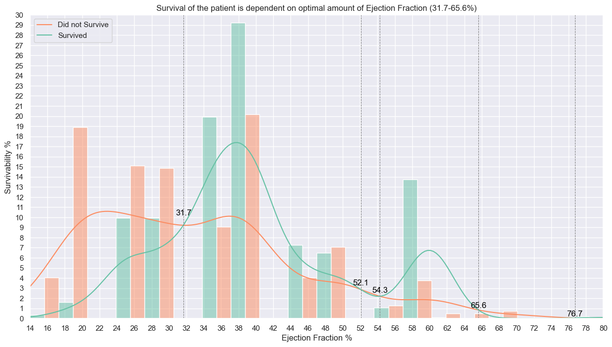
### What is ejection fraction? Ejection fraction refers to how well your heart pumps blood. ### What is a normal ejection fraction? Ejection fraction in a healthy heart is 50% to 70%. With each heartbeat, 50% to 70% of the blood in your left ventricle gets pumped out to your body.

heart_failure_df.groupby(['DEATH_EVENT']).describe()['ejection_fraction'].transpose()
🗸 0.0s

DEATH_EVENT	False	True
count	923.000000	397.000000
mean	39.943662	33.088161
std	10.766355	11.968595
min	17.000000	14.000000
25%	35.000000	25.000000
50%	38.000000	30.000000
75%	45.000000	40.000000
max	80.000000	70.000000

    #ejection_fraction distribution
y_e_f_kde_scale = np.mean(heart_failure_df['ejection_fraction'])*9.5
x_ejection_fraction_intersection_points, y_ejection_fraction_intersection_points, e_f_kde_death_event_0, e_f_kde_death_event_1 = find_kde_intersections(heart_failure_df, 'ejection_fraction', feature_kde_scale=y_e_f_kde_scale)

plt.figure(figsize=(15,8))
plt.title('Survival of the patient is dependent on optimal amount of Ejection Fraction (31.7-65.6%)')

sns.histplot(heart_failure_df,x='ejection_fraction',stat='percent',hue='DEATH_EVENT',palette='Set2',bins=20,kde=True,multiple='dodge',common_norm=False)

plt.xlabel('Ejection Fraction %')
plt.xticks(range(12,81,2))
plt.xlim(14,80)

plt.ylabel('Survivability %')
plt.yticks(range(0,31))
plt.ylim(0,30)

plt.legend(['Did not Survive','Survived'])

for i,x_ejection_fraction_point in enumerate(x_ejection_fraction_intersection_points):
    plt.axvline(x_ejection_fraction_point, color='gray', linestyle='--', linewidth=0.75)
    ef_y_0 = e_f_kde_death_event_0.evaluate(x_ejection_fraction_point)
    ef_y_1 = e_f_kde_death_event_1.evaluate(x_ejection_fraction_point)
    y_value = y_ejection_fraction_intersection_points[i]
    plt.text(x_ejection_fraction_point, y_value, f'{x_ejection_fraction_point:.1f}', color='black', rotation=0,va='bottom', ha='center')

plt.show()
🗸 0.7s

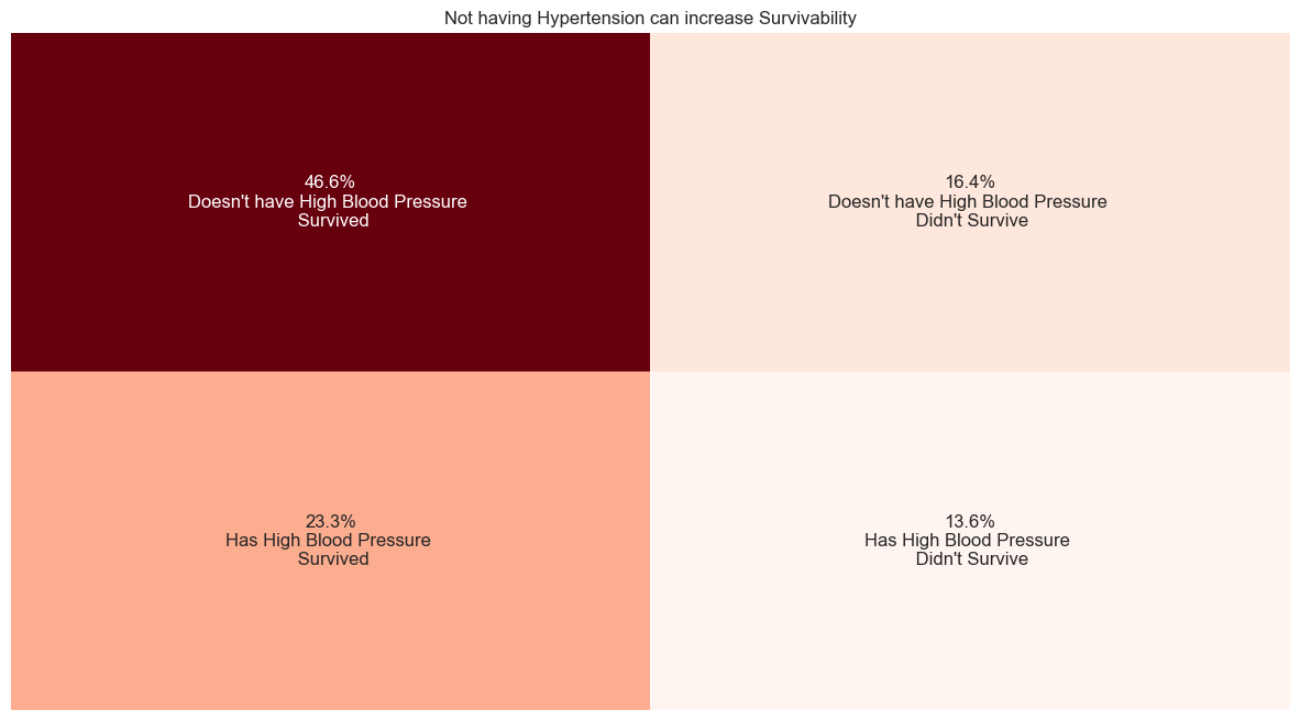
### What is high blood pressure? High blood pressure is when the force of blood pushing against your artery walls is consistently too high. ### How much of our patients have hypertension?

#hypertension distribution
hypertension_contingency_table=pd.crosstab(heart_failure_df['high_blood_pressure'],heart_failure_df['DEATH_EVENT']).copy()

annotations = [
    [
        '{:.1f}%\n{}'.format(hypertension_contingency_table.iloc[i, j] / hypertension_contingency_table.sum().sum() * 100,
                               categorize_values(hypertension_contingency_table.index[i], hypertension_contingency_table.columns[j],'High Blood Pressure'))
        for j in range(len(hypertension_contingency_table.columns))
    ]
    for i in range(len(hypertension_contingency_table.index))
]

plt.figure(figsize=(15,8))
plt.title('Not having Hypertension can increase Survivability')

sns.heatmap(hypertension_contingency_table, annot=annotations, fmt='', cmap='Reds', cbar=False)

plt.xlabel('')
plt.xticks([])

plt.ylabel('')
plt.yticks([])

plt.show()
🗸 0.1s

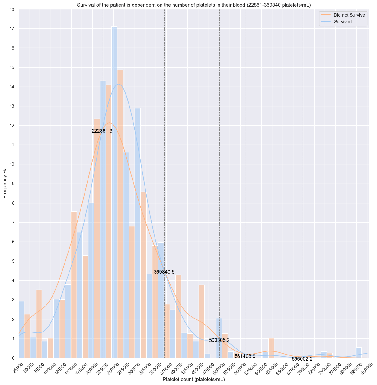
### What are Platelets? Platelets are the cells that circulate within our blood and bind together when they recognize damaged blood vessels. ### What is Normal platelet count range? Normal platelet count ranges from 150,000 to 400,000 platelets/mL

#platelets distribution
y_plt_kde_scale = np.mean(heart_failure_df['platelets'])*10.5
x_platelets_intersection_points, y_platelets_intersection_points, plt_kde_death_event_0, plt_kde_death_event_1 = find_kde_intersections(heart_failure_df, 'platelets', feature_kde_scale=y_plt_kde_scale)

plt.figure(figsize=(15, 15))
plt.title('Survival of the patient is dependent on the number of platelets in their blood (22861-369840 platelets/mL)')

sns.histplot(data=heart_failure_df, x='platelets', hue='DEATH_EVENT',legend=True, stat='percent', kde=True, bins=30,multiple='dodge',common_norm=False)

plt.legend(['Did not Survive','Survived'])

plt.xlabel('Platelet count (platelets/mL)')
plt.xticks(range(25000,855000,25000),rotation=45)
plt.xlim(25000,855000)

plt.ylabel('Frequency %')
plt.yticks(range(0,19))
plt.ylim(0,18)

for i,x_plt_point in enumerate(x_platelets_intersection_points):
    plt.axvline(x_plt_point, color='gray', linestyle='--', linewidth=0.75)
    y_plt_point = y_platelets_intersection_points[i]
    plt.text(x_plt_point, y_plt_point, f'{x_plt_point:.1f}', color='black', rotation=0,va='top', ha='center')

plt.show()
🗸 0.8s

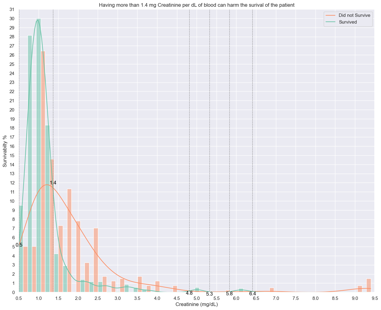
### What is serum creatinine? Creatinine is a waste product in your blood that comes from your muscles. Healthy kidneys filter creatinine out of your blood through your urine. ### What is a normal amount of Creatinine in blood? Normal creatinine levels range from 0.9 to 1.3 mg/dL in men and 0.6 to 1.1 mg/dL in women who are 18 to 60 years old. ### What is the distribution of Creatinine in our patients?

#serum_creatinine distribution
y_crt_kde_scale = np.mean(heart_failure_df['serum_creatinine'])*17.5
x_creatine_intersection_points, y_creatine_intersection_points, crt_kde_death_event_0, crt_kde_death_event_1 = find_kde_intersections(heart_failure_df, 'serum_creatinine', feature_kde_scale=y_crt_kde_scale)

plt.figure(figsize=(15,12))
plt.title('Having more than 1.4 mg Creatinine per dL of blood can harm the surival of the patient')

sns.histplot(heart_failure_df,x='serum_creatinine',stat='percent',hue='DEATH_EVENT',palette='Set2',bins=40,kde=True,multiple='dodge',common_norm=False)

plt.legend(['Did not Survive','Survived'])

plt.xlabel('Creatinine (mg/dL)')
plt.xticks(np.arange(0.5,10,0.5))
plt.xlim(0.5,9.5)

plt.ylabel('Survivabilty %')
plt.yticks(range(0,32))
plt.ylim(0,31)

for i,x_crt_point in enumerate(x_creatine_intersection_points):
    plt.axvline(x_crt_point, color='gray', linestyle='--', linewidth=0.75)
    y_crt_point = y_creatine_intersection_points[i]
    plt.text(x_crt_point, y_crt_point, f'{x_crt_point:.1f}', color='black', rotation=0,va='top', ha='center')

plt.show()
🗸 0.7s

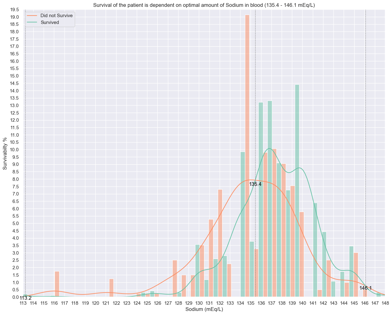
### What is serum sodium? Sodium accounts for approximately 95% of the osmotically active substances in the extracellular compartment, provided that the patient is not in renal failure or does not have severe hyperglycemia. ### What is a normal amount of Sodium in blood? The reference range for serum sodium is 135-147 mEq/L ### What is the distribution of Sodium in our patients?

#serum_sodium distribution
y_sodium_kde_scale = np.mean(heart_failure_df['serum_sodium'])*0.63
x_sodium_intersection_points, y_sodium_intersection_points, sodium_kde_death_event_0, sodium_kde_death_event_1 = find_kde_intersections(heart_failure_df, 'serum_sodium', feature_kde_scale=y_sodium_kde_scale)

plt.figure(figsize=(15,12))
plt.title('Survival of the patient is dependent on optimal amount of Sodium in blood (135.4 - 146.1 mEq/L)')

sns.histplot(heart_failure_df,x='serum_sodium',stat='percent',hue='DEATH_EVENT',palette='Set2',bins=40,kde=True,multiple='dodge',common_norm=False)

plt.legend(['Did not Survive','Survived'])

plt.xlabel('Sodium (mEq/L)')
plt.xticks(range(113,149))
plt.xlim(113,148)

plt.ylabel('Survivabilty %')
plt.yticks(np.arange(0,20,0.5))
plt.ylim(0,19.5)

for i,x_sodium_point in enumerate(x_sodium_intersection_points):
    plt.axvline(x_sodium_point, color='gray', linestyle='--', linewidth=0.75)
    y_sodium_point = y_sodium_intersection_points[i]
    plt.text(x_sodium_point, y_sodium_point, f'{x_sodium_point:.1f}', color='black', rotation=0,va='top', ha='center')

plt.show()
🗸 0.9s

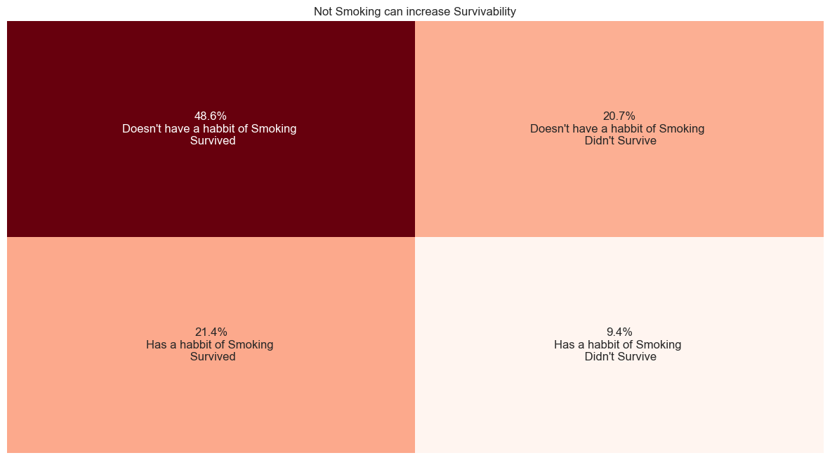
### What percentage of our patients smoke?

#smoking distribution
smoking_contingency_table=pd.crosstab(heart_failure_df['smoking'],heart_failure_df['DEATH_EVENT']).copy()

annotations = [
    [
        '{:.1f}%\n{}'.format(smoking_contingency_table.iloc[i, j] / smoking_contingency_table.sum().sum() * 100,
                             categorize_values(smoking_contingency_table.index[i], smoking_contingency_table.columns[j],'a habbit of Smoking'))
        for j in range(len(smoking_contingency_table.columns))
    ]
    for i in range(len(smoking_contingency_table.index))
]

plt.figure(figsize=(15,8))
plt.title('Not Smoking can increase Survivability')

sns.heatmap(smoking_contingency_table, annot=annotations, fmt='', cmap='Reds', cbar=False)

plt.xlabel('')
plt.xticks([])

plt.ylabel('')
plt.yticks([])

plt.show()
🗸 0.1s

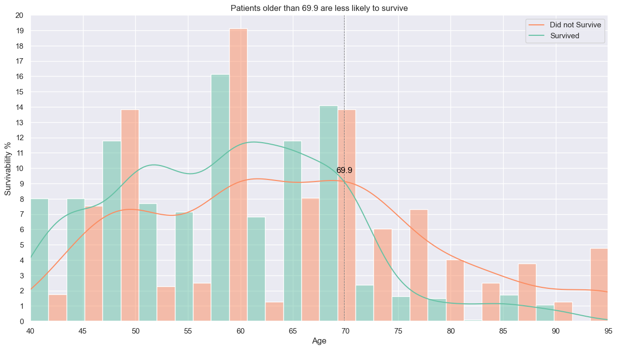
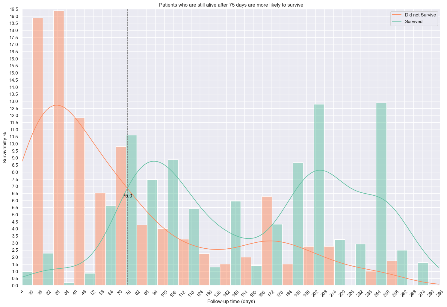
### How did the survivability change during the follow-up period?

#follow-up distribution
y_time_kde_scale = np.mean(heart_failure_df['time'])*10
x_time_intersection_points, y_time_intersection_points, time_kde_death_event_0, time_kde_death_event_1 = find_kde_intersections(heart_failure_df, 'time', feature_kde_scale=y_time_kde_scale)

plt.figure(figsize=(18,12))
plt.title('Patients who are still alive after 75 days are more likely to survive')

sns.histplot(heart_failure_df,x='time',stat='percent',hue='DEATH_EVENT',palette='Set2',bins=20,kde=True,multiple='dodge',common_norm=False)

plt.legend(['Did not Survive','Survived'])

plt.xlabel('Follow-up time (days)')
plt.xticks(range(4,290,6),rotation=45)
plt.xlim(4,286)

plt.ylabel('Survivabilty %')
plt.yticks(np.arange(0,20,0.5))
plt.ylim(0,19.5)

for i,x_time_point in enumerate(x_time_intersection_points):
    plt.axvline(x_time_point, color='gray', linestyle='--', linewidth=0.75)
    y_time_point = y_time_intersection_points[i]
    plt.text(x_time_point, y_time_point, f'{x_time_point:.1f}', color='black', rotation=0,va='top', ha='center')

plt.show()
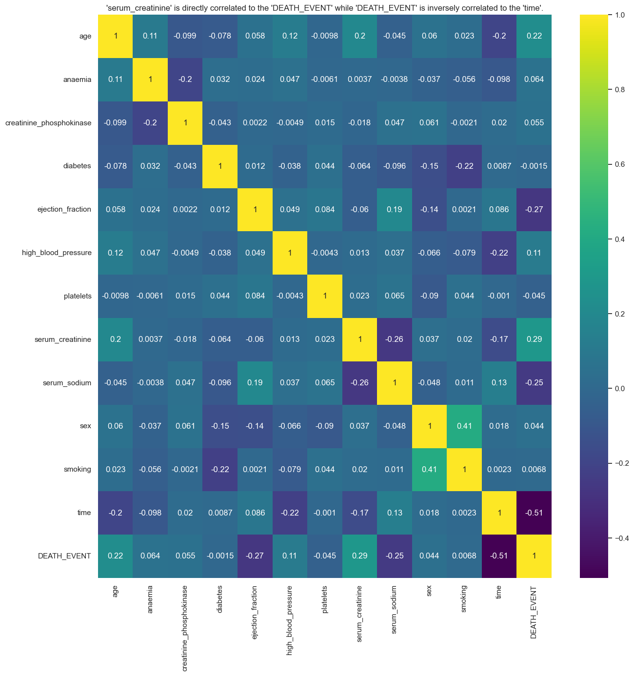
🗸 0.9s
 

#correlation map
plt.figure(figsize=(15,15))
sns.heatmap(heart_failure_df.corr(), annot=True, cmap='viridis')
plt.title("'serum_creatinine' is directly correlated to the 'DEATH_EVENT' while 'DEATH_EVENT' is inversely correlated to the 'time'.")
plt.show()
🗸 0.7s
 

heart_failure_df.describe()
🗸 0.0s

	age	creatinine_phosphokinase	ejection_fraction	platelets	serum_creatinine	serum_sodium	time
count	1320.000000	1320.000000	1320.000000	1320.000000	1320.000000	1320.000000	1320.000000
mean	60.580303	576.135606	37.881818	263751.980303	1.356447	136.665909	132.678788
std	11.913687	970.630878	11.572547	106345.010150	0.998924	4.380990	77.779493
min	40.000000	23.000000	14.000000	25100.000000	0.500000	113.000000	4.000000
25%	50.000000	115.000000	30.000000	208000.000000	0.900000	134.000000	74.000000
50%	60.000000	249.000000	38.000000	263358.000000	1.100000	137.000000	119.500000
75%	69.000000	582.000000	45.000000	310000.000000	1.300000	140.000000	206.000000
max	95.000000	7861.000000	80.000000	850000.000000	9.400000	148.000000	285.000000

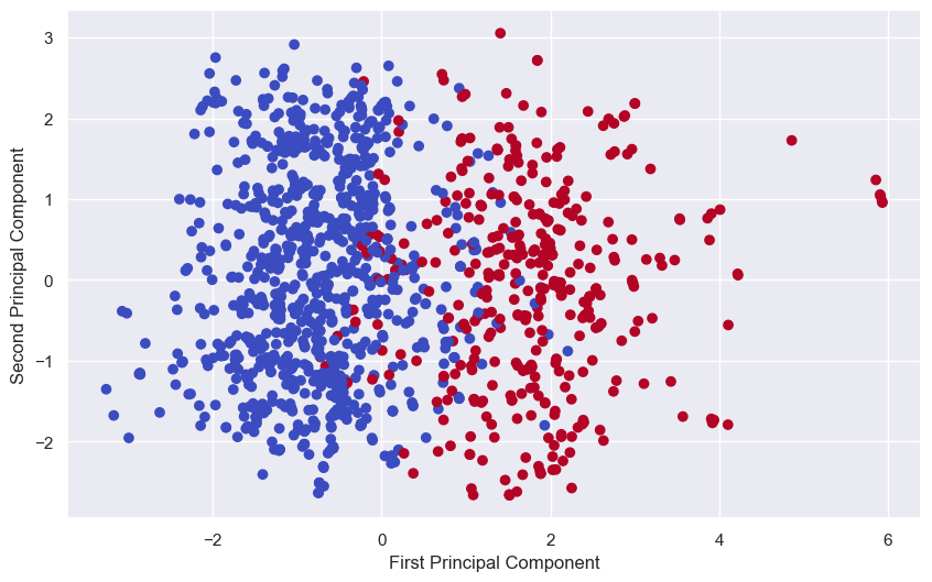
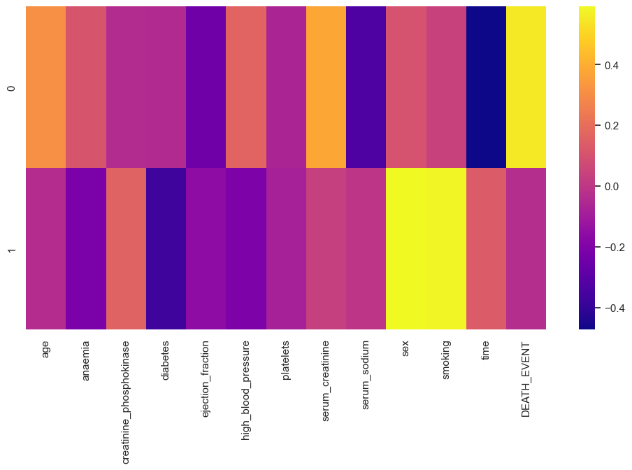
### Principal Component Analysis (PCA)

#### Standardising Dataframe

heart_failure_df.columns
🗸 0.0s Index(['age', 'anaemia', 'creatinine_phosphokinase', 'diabetes',
        'ejection_fraction', 'high_blood_pressure', 'platelets',
        'serum_creatinine', 'serum_sodium', 'sex', 'smoking', 'time',
        'DEATH_EVENT'],
       dtype='object')
    scaler=StandardScaler()
scaler.fit(heart_failure_df)
🗸 0.0s

scaled_data=scaler.transform(heart_failure_df)
pca=PCA(n_components=2)
pca.fit(scaled_data)
    🗸 0.0s

heart_pca=pca.transform(scaled_data)
scaled_data.shape
🗸 0.0s(1320, 13)
    heart_pca.shape
🗸 0.0s(1320, 2)
    plt.figure(figsize=(10,6))
plt.scatter(heart_pca[:,0],heart_pca[:,1],c=heart_failure_df['DEATH_EVENT'],cmap=plt.get_cmap('coolwarm'))
plt.xlabel('First Principal Component')
plt.ylabel('Second Principal Component')
plt.show()
🗸 0.2s
 

pca.components_
    🗸 0.0sarray([[ 0.31246773,  0.11074656, -0.04442332, -0.04853284, -0.24752738,
    0.16718988, -0.06644344,  0.3775265 , -0.33205843,  0.10299891,
    0.04051364, -0.47254404,  0.5511771 ],
  [-0.03804101, -0.21811159,  0.16180196, -0.37501749, -0.15753691,
   -0.20974623, -0.08411439,  0.03326234, -0.00410739,  0.59119629,
    0.58105282,  0.13777242, -0.0321824 ]])
    heart_failure_df_comp=pd.DataFrame(pca.components_,columns=heart_failure_df.columns)
    heart_failure_df_comp
🗸 0.0s

	age	anaemia	creatinine_phosphokinase	diabetes	ejection_fraction	high_blood_pressure	platelets	serum_creatinine	serum_sodium	sex	smoking	time	DEATH_EVENT
0	0.312468	0.110747	-0.044423	-0.048533	-0.247527	0.167190	-0.066443	0.377527	-0.332058	0.102999	0.040514	-0.472544	0.551177
1	-0.038041	-0.218112	0.161802	-0.375017	-0.157537	-0.209746	-0.084114	0.033262	-0.004107	0.591196	0.581053	0.137772	-0.032182

plt.figure(figsize=(12,6))
sns.heatmap(heart_failure_df_comp,cmap='plasma')
plt.show()
🗸 0.4s
 
 From this we can understand that Sex, Smoking, Serum_Creatinine and Age play a major role in the heart organ failure.

## Supervised Learning

X=heart_failure_df.drop(['DEATH_EVENT'],axis=1).copy()
y=heart_failure_df['DEATH_EVENT'].copy()

X_train,X_test,y_train,y_test=train_test_split(X,y,test_size=0.35,random_state=101)

X_train_scaled=scaler.fit_transform(X_train)
🗸 0.0s
X_test_scaled=scaler.transform(X_test)
label_encoder=LabelEncoder()

y_train_encoded=label_encoder.fit_transform(y_train)
y_test_encoded=label_encoder.transform(y_test)
🗸 0.0s

### Logistic Regression

log_model=LogisticRegression()
log_model.fit(X_train_scaled,y_train_encoded)
🗸 0.0s

log_predictions=log_model.predict(X_test_scaled)
print(classification_report(y_test_encoded,log_predictions))
🗸 0.0s
    
        
        precision
        recall
        f1-score
        support
    
    
        0 0.85 0.93 0.89 326
        1 0.79 0.61 0.69 136
        
        accuracy 0.84 462
        macro avg 0.82 0.77 0.79 462
        weighted avg 0.83 0.84 0.83 462
    

print(confusion_matrix(y_test_encoded,log_predictions))
🗸 0.0s [[304  22]
  [ 53  83]]
 log_accuracy=accuracy_score(y_test_encoded, log_predictions)
print(log_accuracy)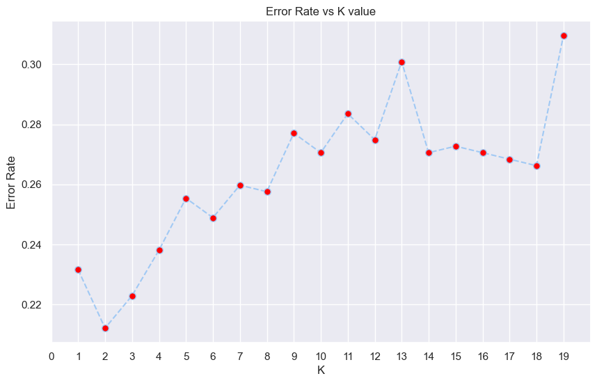
🗸 0.0s 0.8376623376623377

	precision	recall	f1-score	support
0	0.85	0.93	0.89	326
1	0.79	0.61	0.69	136

accuracy			0.84	462
macro avg	0.82	0.77	0.79	462
weighted avg	0.83	0.84	0.83	462

### K-Nearest Neighbour

#### Chosing a K value

error_rate=[]
for i in range (1,20):
    knn_model=KNeighborsClassifier(n_neighbors=i)
    knn_model.fit(X_train,y_train)
    pred_i=knn_model.predict(X_test)
    error_rate.append(np.mean(pred_i!=y_test))
    
plt.figure(figsize=(10,6))
plt.title('Error Rate vs K value')

plt.plot(range(1,20),error_rate,color='b',linestyle='--',marker='o',markerfacecolor='red',markersize=7)

plt.xlabel('K')
plt.xlim(0,20)
plt.xticks(range(0,20,1))

plt.ylabel('Error Rate')

plt.show()
🗸 0.8s
 

knn_model=KNeighborsClassifier(n_neighbors=2)
knn_model.fit(X_train,y_train)
🗸 0.0s


knn_predictions=knn_model.predict(X_test)
print(classification_report(y_test,knn_predictions))
🗸 0.0s
    
        
        precision
        recall
        f1-score
        support
    
    
        False  0.79 0.95 0.86 326
        True 0.76 0.40 0.53 136
        
        accuracy 0.79 462
        macro avg 0.78 0.68 0.70 462
        weighted avg 0.78 0.79 0.76 462
    

print(confusion_matrix(y_test,knn_predictions))
🗸 0.0s [[309  17]
  [ 81  55]]
 knn_accuracy=accuracy_score(y_test, knn_predictions)
print(knn_accuracy)
🗸 0.0s 0.7878787878787878

	precision	recall	f1-score	support
False	0.79	0.95	0.86	326
True	0.76	0.40	0.53	136

accuracy			0.79	462
macro avg	0.78	0.68	0.70	462
weighted avg	0.78	0.79	0.76	462

### Support Vector Machines (SVM)

svc_model=SVC(class_weight='balanced', random_state=42)
svc_model.fit(X_train,y_train)
🗸 0.0s


svc_predictions=svc_model.predict(X_test)
print(classification_report(y_test,svc_predictions))
🗸 0.0s
    
        
        precision
        recall
        f1-score
        support
    
    
        False 0.72 0.71 0.71 326
        True 0.32 0.33 0.33 136
        
        accuracy 0.60 462
        macro avg 0.52 0.52 0.52 462
        weighted avg 0.60 0.60 0.60 462
    

print(confusion_matrix(y_test,svc_predictions))
🗸 0.0s [[231  95]
  [ 91  45]]
 svc_accuracy=accuracy_score(y_test, svc_predictions)
print(svc_accuracy)
🗸 0.0s 0.5974025974025974

	precision	recall	f1-score	support
False	0.72	0.71	0.71	326
True	0.32	0.33	0.33	136

accuracy			0.60	462
macro avg	0.52	0.52	0.52	462
weighted avg	0.60	0.60	0.60	462

#### SVC with SMOTE

smote = SMOTE(random_state=101)
X_train_res, y_train_res = smote.fit_resample(X_train, y_train)
svc_model_new = SVC(random_state=101)
svc_model_new.fit(X_train_res,y_train_res)
🗸 0.0s


svc_predictions_new = svc_model_new.predict(X_test)
print(classification_report(y_test,svc_predictions_new))
🗸 0.0s
    
        
        precision
        recall
        f1-score
        support
    
    
        False 0.72 0.74 0.73 326
        True 0.33 0.30 0.31 136
        
        accuracy 0.61 462
        macro avg 0.52 0.52 0.52 462
        weighted avg 0.60 0.61 0.61 462
    

print(confusion_matrix(y_test,svc_predictions_new))
🗸 0.0s [[242  84]
  [ 95  41]]
 svc_accuracy_new=accuracy_score(y_test, svc_predictions_new)
print(svc_accuracy_new)
🗸 0.0s 0.6125541125541125

	precision	recall	f1-score	support
False	0.72	0.74	0.73	326
True	0.33	0.30	0.31	136

accuracy			0.61	462
macro avg	0.52	0.52	0.52	462
weighted avg	0.60	0.61	0.61	462

#### Grid-search SVM

param_grid={'C':[0.1,1,10,100,1000],'gamma':[1,0.1,0.01,0.001,0.0001]}
grid_model=GridSearchCV(SVC(),param_grid,verbose=3)
grid_model.fit(X_train,y_train)
🗸 7.8s Fitting 5 folds for each of 25 candidates, totalling 125 fits
 [CV 1/5] END ....................C=0.1, gamma=1;, score=0.692 total time=   0.0s
 [CV 2/5] END ....................C=0.1, gamma=1;, score=0.698 total time=   0.0s
 [CV 3/5] END ....................C=0.1, gamma=1;, score=0.698 total time=   0.0s
 [CV 4/5] END ....................C=0.1, gamma=1;, score=0.696 total time=   0.0s
 [CV 5/5] END ....................C=0.1, gamma=1;, score=0.696 total time=   0.0s
 [CV 1/5] END ..................C=0.1, gamma=0.1;, score=0.692 total time=   0.0s
 [CV 2/5] END ..................C=0.1, gamma=0.1;, score=0.698 total time=   0.0s
 [CV 3/5] END ..................C=0.1, gamma=0.1;, score=0.698 total time=   0.0s
 [CV 4/5] END ..................C=0.1, gamma=0.1;, score=0.696 total time=   0.0s
 [CV 5/5] END ..................C=0.1, gamma=0.1;, score=0.696 total time=   0.0s
 [CV 1/5] END .................C=0.1, gamma=0.01;, score=0.692 total time=   0.0s
 [CV 2/5] END .................C=0.1, gamma=0.01;, score=0.698 total time=   0.0s
 [CV 3/5] END .................C=0.1, gamma=0.01;, score=0.698 total time=   0.0s
 [CV 4/5] END .................C=0.1, gamma=0.01;, score=0.696 total time=   0.0s
 [CV 5/5] END .................C=0.1, gamma=0.01;, score=0.696 total time=   0.0s
 [CV 1/5] END ................C=0.1, gamma=0.001;, score=0.692 total time=   0.0s
 [CV 2/5] END ................C=0.1, gamma=0.001;, score=0.698 total time=   0.0s
 [CV 3/5] END ................C=0.1, gamma=0.001;, score=0.698 total time=   0.0s
 [CV 4/5] END ................C=0.1, gamma=0.001;, score=0.696 total time=   0.0s
 [CV 5/5] END ................C=0.1, gamma=0.001;, score=0.696 total time=   0.0s
 [CV 1/5] END ...............C=0.1, gamma=0.0001;, score=0.692 total time=   0.0s
 [CV 2/5] END ...............C=0.1, gamma=0.0001;, score=0.698 total time=   0.0s
 [CV 3/5] END ...............C=0.1, gamma=0.0001;, score=0.698 total time=   0.0s
 [CV 4/5] END ...............C=0.1, gamma=0.0001;, score=0.696 total time=   0.0s
 ...
 [CV 2/5] END ..............C=1000, gamma=0.0001;, score=0.785 total time=   0.0s
 [CV 3/5] END ..............C=1000, gamma=0.0001;, score=0.733 total time=   0.0s
 [CV 4/5] END ..............C=1000, gamma=0.0001;, score=0.749 total time=   0.0s
 [CV 5/5] END ..............C=1000, gamma=0.0001;, score=0.754 total time=   0.0s
 Output is truncated. View as a scrollable element or open in a text editor. Adjust cell output settings...


grid_predictions=grid_model.predict(X_test)
print(classification_report(y_test,grid_predictions))
🗸 0.0s
    
        
        precision
        recall
        f1-score
        support
    
    
        False 0.80 0.94 0.86 326
        True 0.74 0.44 0.55 136
        
        accuracy 0.79 462
         macro avg 0.77 0.69 0.71 462
        weighted avg 0.78 0.79 0.77 462
    

print(confusion_matrix(y_test,grid_predictions))
🗸 0.0s [[305  21]
  [ 76  60]]
 grid_accuracy=accuracy_score(y_test, grid_predictions)
print(grid_accuracy)
🗸 0.0s 0.79004329004329

	precision	recall	f1-score	support
False	0.80	0.94	0.86	326
True	0.74	0.44	0.55	136

accuracy			0.79	462
macro avg	0.77	0.69	0.71	462
weighted avg	0.78	0.79	0.77	462

### K-Means Clustering

kmeans_model=KMeans(n_clusters=2,n_init=50)
kmeans_model.fit(X)
🗸 0.4s

print(confusion_matrix(y,kmeans_model.labels_))
🗸 0.0s [[332 591]
  [128 269]]
print(classification_report(y,kmeans_model.labels_))
🗸 0.0s
    
        
        precision
        recall
        f1-score
        support
    
    
        False 0.72 0.36 0.48 923
        True 0.31 0.68 0.43 397
        
        accuracy 0.46 1320
        macro avg  0.52 0.52 0.45 1320
        weighted avg  0.60 0.46 0.46 1320
    

 kmeans_accuracy=accuracy_score(y, kmeans_model.labels_)
print(kmeans_accuracy)
🗸 0.0s 0.4553030303030303

	precision	recall	f1-score	support
False	0.72	0.36	0.48	923
True	0.31	0.68	0.43	397

accuracy			0.46	1320
macro avg	0.52	0.52	0.45	1320
weighted avg	0.60	0.46	0.46	1320

### Decision Tree Model

dtree_model=DecisionTreeClassifier()
dtree_model.fit(X_train,y_train)
🗸 0.4s

dtree_prediction=dtree_model.predict(X_test)
print(classification_report(y_test,dtree_prediction))
🗸 0.0s
    
        
        precision
        recall
        f1-score
        support
    
    
        False 0.94 0.95 0.95 326
        True 0.88 0.86 0.87 136
        
        accuracy 0.92 462
        macro avg 0.91 0.91 0.91 462
        weighted avg 0.92 0.92 0.92 462
    

print(confusion_matrix(y_test,dtree_prediction))
🗸 0.0s [[310  16]
  [19 117]]
 dtree_accuracy=accuracy_score(y_test, dtree_prediction)
print(dtree_accuracy)
🗸 0.0s 0.9242424242424242

	precision	recall	f1-score	support
False	0.94	0.95	0.95	326
True	0.88	0.86	0.87	136

accuracy			0.92	462
macro avg	0.91	0.91	0.91	462
weighted avg	0.92	0.92	0.92	462

### Random Forest Classifier

rfc_model=RandomForestClassifier(n_estimators=250)
rfc_model.fit(X_train,y_train)
🗸 0.4s

rfc_prediction=rfc_model.predict(X_test)
print(classification_report(y_test,rfc_prediction))
🗸 0.0s
    
        
        precision
        recall
        f1-score
        support
    
    
        False 0.94 0.98 0.96 326
        True 0.94 0.85 0.90 136
        
        accuracy 0.94 462
        macro avg 0.94 0.92 0.93 462
        weighted avg 0.94 0.94 0.94 462
    

print(confusion_matrix(y_test,rfc_prediction))
🗸 0.0s [[319  7]
  [20 116]]
 rfc_accuracy=accuracy_score(y_test, rfc_prediction)
print(rfc_accuracy)
🗸 0.0s 0.9415584415584416

	precision	recall	f1-score	support
False	0.94	0.98	0.96	326
True	0.94	0.85	0.90	136

accuracy			0.94	462
macro avg	0.94	0.92	0.93	462
weighted avg	0.94	0.94	0.94	462

### Naive Bayes

nb_model=GaussianNB()
nb_model.fit(X_train,y_train)
🗸 0.0s

nb_prediction=nb_model.predict(X_test)
print(classification_report(y_test,nb_prediction))
🗸 0.0s
    
        
        precision
        recall
        f1-score
        support
    
    
        False 0.81 0.96 0.88 326
        True 0.84 0.46 0.59 136
        
        accuracy 0.81 462
        macro avg 0.82 0.71 0.74 462
        weighted avg 0.82 0.81 0.79 462
    

print(confusion_matrix(y_test,nb_prediction))
🗸 0.0s [[314  12]
  [74 62]]
 nb_accuracy=accuracy_score(y_test, nb_prediction)
print(nb_accuracy)
🗸 0.0s 0.8138528138528138

	precision	recall	f1-score	support
False	0.81	0.96	0.88	326
True	0.84	0.46	0.59	136

accuracy			0.81	462
macro avg	0.82	0.71	0.74	462
weighted avg	0.82	0.81	0.79	462

### XGBoost

xgb_train=xgb.DMatrix(X_train,label=y_train)
xgb_test=xgb.DMatrix(X_test,label=y_test)
🗸 0.2s
num_round=100
parameters={
     'max_depth':6,
     'eta':0.3,
     'objective':'binary:logistic',
     'eval_metric':'logloss'
     }
watchlist=[(xgb_train,'train'),(xgb_test,'eval')]
xgb_model=xgb.train(params=parameters,dtrain=xgb_train,num_boost_round=num_round,evals=watchlist,early_stopping_rounds=10)
🗸 0.2s [0]	train-logloss:0.44851	eval-logloss:0.45720
 [1]	train-logloss:0.35219	eval-logloss:0.38021
 [2]	train-logloss:0.28499	eval-logloss:0.32778
 [3]	train-logloss:0.23488	eval-logloss:0.28703
 [4]	train-logloss:0.20022	eval-logloss:0.26685
 [5]	train-logloss:0.17326	eval-logloss:0.24388
 [6]	train-logloss:0.15428	eval-logloss:0.22823
 [7]	train-logloss:0.13900	eval-logloss:0.21794
 [8]	train-logloss:0.12655	eval-logloss:0.20990
 [9]	train-logloss:0.11059	eval-logloss:0.19332
 [10]	train-logloss:0.09777	eval-logloss:0.18444
 [11]	train-logloss:0.09057	eval-logloss:0.18123
 [12]	train-logloss:0.08555	eval-logloss:0.17707
 [13]	train-logloss:0.07857	eval-logloss:0.17370
 [14]	train-logloss:0.07205	eval-logloss:0.16914
 [15]	train-logloss:0.06748	eval-logloss:0.16586
 [16]	train-logloss:0.06481	eval-logloss:0.16455
 [17]	train-logloss:0.06135	eval-logloss:0.16109
 [18]	train-logloss:0.05941	eval-logloss:0.15921
 [19]	train-logloss:0.05713	eval-logloss:0.15679
 [20]	train-logloss:0.05443	eval-logloss:0.15525
 [21]	train-logloss:0.05062	eval-logloss:0.15221
 [22]	train-logloss:0.04771	eval-logloss:0.15274
 [23]	train-logloss:0.04650	eval-logloss:0.15195
 [24]	train-logloss:0.04387	eval-logloss:0.15039
 [25]	train-logloss:0.04204	eval-logloss:0.15247
 [26]	train-logloss:0.04017	eval-logloss:0.15135
 ...
 [65]	train-logloss:0.01707	eval-logloss:0.14778
 [66]	train-logloss:0.01689	eval-logloss:0.14785
 [67]	train-logloss:0.01666	eval-logloss:0.14841
 [68]	train-logloss:0.01653	eval-logloss:0.14881
 Output is truncated. View as a scrollable element or open in a text editor. Adjust cell output settings...
    xgb_prediction_prob=xgb_model.predict(xgb_test)
xgb_prediction=(xgb_prediction_prob > 0.5).astype(int)
print(classification_report(y_test,xgb_prediction))
🗸 0.0s
    
        
        precision
        recall
        f1-score
        support
    
    
        False 0.96 0.98 0.97 326
        True 0.95 0.89 0.92 136
        
        accuracy 0.95 462
        macro avg 0.95 0.93 0.94 462
        weighted avg 0.95 0.95 0.95 462
    

print(confusion_matrix(y_test,nb_prediction))
🗸 0.0s [[319  7]
  [15 121]]
 xgb_accuracy=accuracy_score(y_test, xgb_prediction)
print(xgb_accuracy)
🗸 0.0s 0.9523809523809523

	precision	recall	f1-score	support
False	0.96	0.98	0.97	326
True	0.95	0.89	0.92	136

accuracy			0.95	462
macro avg	0.95	0.93	0.94	462
weighted avg	0.95	0.95	0.95	462

## So to recap, we used supervised learning to predict the probability of a patient's death occuring. We used the following methods to do it. * Naive Bayes Classifier * K-Nearest Neighbour * Logistic Regression * Random Forest Classifier * Support Vector Machines (SVM) * Support Vector Machines (SVM) using Synthetic Minority Oversampling Technique (SMOTE) * Support Vector Machines (SVM) using GridSearchCV * K-Means Clustering * Decision Tree Model * XGBoost Classifier

xgb_train=xgb.DMatrix(X_train,label=y_train)
xgb_test=xgb.DMatrix(X_test,label=y_test)
🗸 0.2s
prediction_accuracies={
    nb_accuracy:"Gaussian Naive Bayes Classifier",
    knn_accuracy:"K-Nearest Neighbour Classifier",
    log_accuracy:"Logistic Regression Model",
    rfc_accuracy:"Random Forest Classifier",
    svc_accuracy:"Support Vector Machines (SVM)",
    svc_accuracy_new:"Support Vector Machines (SVM) using Synthetic Minority Oversampling Technique (SMOTE)",
    grid_accuracy:"Support Vector Machines (SVM) using GridSearchCV",
    dtree_accuracy:"Decision Tree Model",
    kmeans_accuracy:"K-Means Clustering",
    xgb_accuracy:'XGBoost Classifier'
}
max_accuracy=max(prediction_accuracies)
most_accurate_model=prediction_accuracies[max_accuracy]
print(f'The Most accurate model is {most_accurate_model} with {round(max_accuracy*100,2)}% accuracy')
🗸 0.0s The Most accurate model is XGBoost Classifier with 95.24% accuracy

Heart Failure Prediction by Analysing Clinical Records

Dataset

Code

Email

Phone

Address